Digital forensics

Geocoding Router Log Data

Any good piece of malware eventually has to phone home. What good is collecting your dirty little secrets if it can't capitalize on them? This article will help demonstrate how a little bit of forensic analysis can help you visualize where your data is going.

Learn Digital Forensics

Build your skills with hands-on forensics training for computers, mobile devices, networks and more.

Start Learning

Web site access logs are often used for web analytics. These logs can be sliced and diced to determine where visitors are coming from, when they're visiting, what they're looking at, and what browsers they're using. That's all very useful. Malware doesn't want to be so useful; it wants to be as stealthy and unobtrusive as possible. Malware is a pickpocket.

After malware is done logging your keystrokes, gathering your credentials, or collecting whatever it wants to collect, it needs to do something with that data. Many times, it's a quick TCP connection home. Your firewall won't catch the connection, because the malware makes a legitimate HTTP request. Your DLP won't catch it, because the malware is smart and uses SSL to encrypt the outgoing traffic. While you may not be able to catch it red-handed, you can still do something about it after the fact.

You can extract IP addresses from your router logs (routers, proxies, wherever you capture this information) and analyze outbound connections and visualize--using maps!--where your data is going. Why maps? Because maps get the attention of your organization's managers.

Sweet! How?

There's the easy way and there's the hard way. The easy way involves some manual processes that I'll use to demonstrate the process; the hard way involves automating and customizing these processes to suit your needs. I'll go over the easy way and leave the hard way up to you.

The steps are straightforward:

1. Extract IP addresses from your logs.
   
2. Format the IP addresses.
   
3. Visualize the IP addresses.
   
4. Sit back and enjoy the admiration of your colleagues and managers.
   

Step 1: Extract the IP addresses

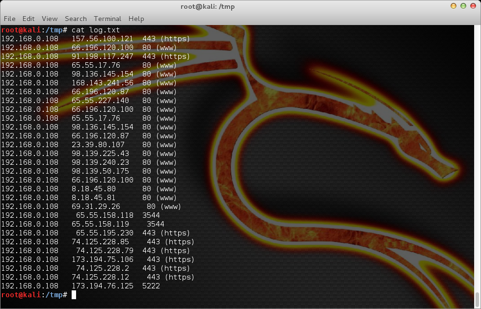
Your log file might look something like this:

[plain]

192.168.0.108 157.56.100.121 443 (https)

192.168.0.108 66.196.120.100 80 (www)

192.168.0.108 91.198.117.247 443 (https)

192.168.0.108 65.55.17.76 80 (www)

192.168.0.108 98.136.145.154 80 (www)

192.168.0.108 168.143.241.56 80 (www)

192.168.0.108 66.196.120.87 80 (www)

192.168.0.108 65.55.227.140 80 (www)

192.168.0.108 66.196.120.100 80 (www)

192.168.0.108 65.55.17.76 80 (www)

192.168.0.108 98.136.145.154 80 (www)

192.168.0.108 66.196.120.87 80 (www)

192.168.0.108 23.39.80.107 80 (www)

192.168.0.108 98.139.225.43 80 (www)

192.168.0.108 98.139.240.23 80 (www)

192.168.0.108 98.139.50.175 80 (www)

192.168.0.108 66.196.120.100 80 (www)

192.168.0.108 8.18.45.80 80 (www)

192.168.0.108 8.18.45.81 80 (www)

192.168.0.108 69.31.29.26 80 (www)

192.168.0.108 65.55.158.118 3544

192.168.0.108 65.55.158.119 3544

192.168.0.108 65.55.195.230 443 (https)

192.168.0.108 74.125.228.85 443 (https)

192.168.0.108 74.125.228.79 443 (https)

192.168.0.108 173.194.75.106 443 (https)

192.168.0.108 74.125.228.2 443 (https)

192.168.0.108 74.125.228.12 443 (https)

192.168.0.108 173.194.76.125 5222

[/plain]

In this case, the router displays the source IP address (where the request came from), the destination IP address (where the request is going), and the port (what the destination application is).

Step 2: Format the IP addresses

We're going to format these addresses to better suit our needs. For the purposes of this demonstration, we're just going to need the IP address and port of each request. Assuming we store the log file in "log.txt," we can use awk to format the data as we need to:

cat log.txt | awk 'BEGIN {OFS="t"; print "IP", "Port"} {print $2, $3} END {}'

which renders:

[plain]

IP Port

157.56.100.121 443

66.196.120.100 80

91.198.117.247 443

65.55.17.76 80

98.136.145.154 80

168.143.241.56 80

66.196.120.87 80

65.55.227.140 80

66.196.120.100 80

65.55.17.76 80

98.136.145.154 80

66.196.120.87 80

23.39.80.107 80

98.139.225.43 80

98.139.240.23 80

98.139.50.175 80

66.196.120.100 80

8.18.45.80 80

8.18.45.81 80

69.31.29.26 80

65.55.158.118 3544

65.55.158.119 3544

65.55.195.230 443

74.125.228.85 443

74.125.228.79 443

173.194.75.106 443

74.125.228.2 443

74.125.228.12 443

173.194.76.125 5222

[/plain]

First, a quick note on awk. Any number of tools (perl, sed, etc.) can be used to parse the output, but awk serves the purpose as well as any. It accepts the output piped to it from the "cat" command and extracts only the second and third columns (IP and port, respectively) and displays them in two tab-delimited columns. Here is the syntax:

Step 3: Visualize the IP addresses

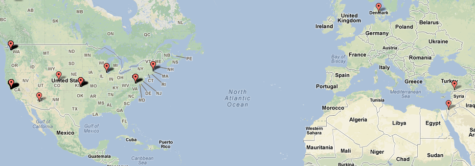
Here's where things get fun. Now that we have the address and port information formatted correctly, we'll use BatchGeo to visualize the data. This site will geocode the IP address locations and plot each one on a map. We simply copy the IP and port data and then paste it into BatchGeo's interface. Using its options, we will also color-code each address by port, thereby giving us an at-a-glance representation of each service/application.

Next, click the "Make Map" button to make the magic happen:

Step 4: Sit back and enjoy the admiration of your colleagues and managers

Looking at this map, a couple of things really jump out. First, Greenland looks really big (and not very green). Second, there are two IP address where I wouldn't have expected: one in Turkey and one in Israel. Doing a search on TCPIPUTILS.com, I see that each of those addresses is associated with spyware. (It should be noted that TCPIPUTILS.com actually locates this address in New York City. This discrepancy underscores that suspect addresses should be further validated to ensure accuracy.)

The color groups show that most outbound traffic is using HTTP. Outbound connections using unexpected ports should be further investigated. My map uses the following colors:

Other uses:

• Add a map marker attribute to display IP address that originated the request.
  
• Parse the output of netstat to visualize active connections and display the process name for each connection.
  
• Create color groups of outbound connections by time to see where after-hours traffic is going.
  
• Perform the same analysis on your web server access logs.
  

Conclusion

Remember, this is the "easy" way, in that I'm doing everything here manually to demonstrate the process and capabilities. There are ways to automate this, obviously. BatchGeo offers a friendly way to quickly visualize the data. For greater flexibility, you could use a service like http://freegeoip.net to look up the geocodes of IP addresses and leverage the Google Maps API (http://maps.google.com/maps/api) to create your own map markers.

References:

https://code.google.com/p/apachegeomap/

http://www.batchgeo.com

http://www.tcpiputils.com/browse/ip-address

Learn Digital Forensics

Build your skills with hands-on forensics training for computers, mobile devices, networks and more.

Start Learning

http://freegeoip.net/